Tutorial 
- Tutorial
Tutorial
This chapter contains a short overview of igraph’s capabilities. It is highly recommended to read it at least once if you are new to igraph. I assume that you have already installed igraph; if you did not, see Installing igraph first. Familiarity with the Python language is also assumed; if this is the first time you are trying to use Python, there are many good Python tutorials on the Internet to get you started. If this is the first time you ever try to use a programming language, A Byte of Python is a good place to start out. If you already have a stable programming background in other languages and you just want a quick overview of Python, Learn Python in 10 minutes is probably your best bet.
Starting igraph
igraph is a Python module, hence it can be imported exactly the same way as any other ordinary Python module at the Python prompt:
$ python
Python 3.9.6 (default, Jun 29 2021, 05:25:02)
[Clang 12.0.5 (clang-1205.0.22.9)] on darwin
Type "help", "copyright", "credits" or "license" for more information.
>>> import igraph
This imports igraph’s objects and methods inside an own namespace called igraph. Whenever
you would like to call any of igraph’s methods, you will have to provide the appropriate
namespace-qualification. E.g., to check which igraph version you are using, you could do the
following:
>>> import igraph
>>> print(igraph.__version__)
0.9.6
Another way to make use of igraph is to import all its objects and methods into the main Python namespace (so you do not have to type the namespace-qualification every time). This is fine as long as your own objects and methods do not conflict with the ones provided by igraph:
>>> from igraph import *
The third way to start igraph is to simply call the startup script that was supplied with
the igraph package you installed. Not too surprisingly, the script is called igraph,
and provided that the script is on your path in the command line of your operating system
(which is almost surely the case on Linux and OS X), you can simply type igraph at the
command line. Windows users will find the script inside the scripts subdirectory of Python
and you may have to add it manually to your path in order to be able to use the script from
the command line without typing the whole path.
When you start the script, you will see something like this:
$ igraph
No configuration file, using defaults
igraph 0.9.6 running inside Python 3.9.6 (default, Jun 29 2021, 05:25:02)
Type "copyright", "credits" or "license" for more information.
>>>
The command-line startup script imports all of igraph’s methods and objects into the main
namespace, so it is practically equivalent to from igraph import *. The difference between
the two approaches (apart from saving some typing) is that the command-line script checks
whether you have any of Python’s more advanced shells installed and uses that instead of the
standard Python shell. Currently the module looks for IPython and
IDLE (the Tcl/Tk-based graphical shell supplied with Python). If neither IPython nor IDLE is
installed, the startup script launches the default Python shell. You can also modify the
order in which these shells are searched by tweaking igraph’s configuration file
(see configuring-igraph).
In general, it is advised to use the command line startup script when using igraph
interactively (i.e., when you just want to quickly load or generate some graphs, calculate
some basic properties and save the results somewhere). For non-disposable graph analysis
routines that you intend to re-run from time to time, you should write a script separately
in a .py source file and import igraph using one of the above methods at the start of
the script, then launch the script using the Python interpreter.
From now on, every example in the documentation will assume that igraph’s objects and
methods are imported into the main namespace (i.e., we used from igraph import *
instead of import igraph). If you let igraph take its own namespace, please adjust
all the examples accordingly.
Creating a graph from scratch
Assuming that you have started igraph successfully, it is time to create your first igraph graph. This is pretty simple:
>>> g = Graph()
The above statement created an undirected graph with no vertices or edges and assigned it to the variable g. To confirm that it’s really an igraph graph, we can print it:
>>> g
<igraph.Graph object at 0x4c87a0>
This tells us that g is an instance of igraph’s Graph class and
that it is currently living at the memory address 0x4c87a0 (the exact
output will almost surely be different for your platform). To obtain a more
user-friendly output, we can try to print the graph using Python’s
print statement:
>>> print(g)
IGRAPH U--- 0 0 --
This summary consists of IGRAPH, followed by a four-character long code, the number of vertices, the number of edges, two dashes (–) and the name of the graph (i.e. the contents of the name attribute, if any)
This is not too exciting so far; a graph with no vertices and no edges is not really useful for us. Let’s add some vertices first!
>>> g.add_vertices(3)
Graph.add_vertices() (i.e., the add_vertices() method of the Graph
class) adds the given number of vertices to the graph.
Now our graph has three vertices but no edges, so let’s add some edges as well! You can
add edges by calling Graph.add_edges() - but in order to add edges, you have to refer to
existing vertices somehow. igraph uses integer vertex IDs starting from zero, thus the
first vertex of your graph has index zero, the second vertex has index 1 and so on.
Edges are specified by pairs of integers, so [(0,1), (1,2)] denotes a list of two
edges: one between the first and the second, and the other one between the second and the
third vertices of the graph. Passing this list to Graph.add_edges() adds these two edges
to your graph:
>>> g.add_edges([(0,1), (1,2)])
add_edges() is clever enough to figure out what you want to do in most of the
cases: if you supply a single pair of integers, it will automatically assume that you want
to add a single edge. However, if you try to add edges to vertices with invalid IDs (i.e.,
you try to add an edge to vertex 5 when you only have three vertices), you will get an
exception:
>>> g.add_edges((5, 0))
Traceback (most recent call last):
  File "<stdin>", line 6, in <module>
TypeError: iterable must return pairs of integers or strings
Most igraph functions will raise an igraph.InternalError if
something goes wrong. The message corresponding to the exception gives you a
short textual explanation of what went wrong (cannot add edges, invalid
vertex id) along with the corresponding line in the C source where the error
occurred. The exact filename and line number may not be too informative to you,
but it is invaluable for igraph developers if you think you found an error in
igraph and you want to report it.
Let us go on with our graph g and add some more vertices and edges to it:
>>> g.add_edges([(2, 0)])
>>> g.add_vertices(3)
>>> g.add_edges([(2, 3), (3, 4), (4, 5), (5, 3)])
>>> print(g)
IGRAPH U---- 6 7 --
+ edges:
0--1 1--2 0--2 2--3 3--4 4--5 3--5
Now, this is better. We have an undirected graph with six vertices and seven
edges, and you can also see the list of edges in igraph’s output. Edges also
have IDs, similarly to vertices; they also start from zero and edges that were
added later have higher IDs than edges that were added earlier. Vertex and edge
IDs are always continuous, and a direct consequence of this fact is that if
you happen to delete an edge, chances are that some (or all) of the edges will
be renumbered. Moreover, if you delete a vertex, even the vertex IDs will
change. Edges can be deleted by delete_edges() and it requires a
list of edge IDs to be deleted (or a single edge ID). Vertices can be deleted
by delete_vertices() and you may have already guessed that it
requires a list of vertex IDs to be deleted (or a single vertex ID). If you do
not know the ID of an edge you wish to delete, but you know the IDs of the
vertices at its two endpoints, you can use get_eid() to get the
edge ID. Remember, all these are methods of the Graph class and you
must call them on the appropriate Graph instance!
>>> g.get_eid(2, 3)
3
>>> g.delete_edges(3)
>>> summary(g)
IGRAPH U--- 6 6 --
summary() is a new command that you haven’t seen before; it is a member of igraph’s
own namespace and it can be used to get an overview of a given graph object. Its output
is similar to the output of print but it does not print the edge list to avoid
cluttering up the display for large graphs. In general, you should use summary()
instead of print when working interactively with large graphs because printing the
edge list of a graph with millions of vertices and edges could take quite a lot of time.
Generating graphs
igraph includes a large set of graph generators which can be divided into two groups: deterministic and stochastic graph generators. Deterministic generators produce the same graph if you call them with exactly the same parameters, while stochastic generators produce a different graph every time. Deterministic generators include methods for creating trees, regular lattices, rings, extended chordal rings, several famous graphs and so on, while stochastic generators are used to create Erdős-Rényi random networks, Barabási-Albert networks, geometric random graphs and such. igraph has too many generators to cover them all in this tutorial, so we will only try a deterministic and a stochastic generator instead:
>>> g = Graph.Tree(127, 2)
>>> summary(g)
IGRAPH U--- 127 126 --
Graph.Tree() generates a regular tree graph. The one that we generated has 127
vertices and each vertex (apart from the leaves) has two children (and of course one
parent). No matter how many times you call Graph.Tree(), the generated graph will
always be the same if you use the same parameters:
>>> g2 = Graph.Tree(127, 2)
>>> g2.get_edgelist() == g.get_edgelist()
True
The above code snippet also shows you that the get_edgelist() method
of Graph graph objects return a list that contains pairs of integers, one for
each edge. The first member of the pair is the source vertex ID and the second member
is the target vertex ID of the corresponding edge. This list is too long, so let’s
just print the first 10 elements!
>>> g2.get_edgelist()[0:10]
[(0, 1), (0, 2), (1, 3), (1, 4), (2, 5), (2, 6), (3, 7), (3, 8), (4, 9), (4, 10)]
Let’s do the same with a stochastic generator!
>>> g = Graph.GRG(100, 0.2)
>>> summary(g)
IGRAPH U---- 100 516 --
+ attr: x (v), y (v)
where + attr shows names of the attributes for vertices (v) and edges (e).
Graph.GRG() generates a geometric random graph: n points are chosen randomly and
uniformly inside the unit square and pairs of points closer to each other than a predefined
distance d are connected by an edge. In our case, n is 100 and d is 0.2. Due to
the random nature of the algorithm, chances are that the exact graph you got is different
from the one that was generated when I wrote this tutorial, hence the values above in the
summary will not match the ones you got. This is normal and expected. Even if you generate
two geometric random graphs on the same machine, they will be different for the same parameter
set:
>>> g2 = Graph.GRG(100, 0.2)
>>> g.get_edgelist() == g2.get_edgelist()
False
>>> g.isomorphic(g2)
False
isomorphic() tells you whether two graphs are isomorphic or not. In general,
it might take quite a lot of time, especially for large graphs, but in our case, the
answer can quickly be given by checking the degree distributions of the two graphs.
Setting and retrieving attributes
igraph uses vertex and edge IDs in its core. These IDs are integers, starting from zero,
and they are always continuous at any given time instance during the lifetime of the graph.
This means that whenever vertices and edges are deleted, a large set of edge and possibly
vertex IDs will be renumbered to ensure the continuity. Now, let us assume that our graph
is a social network where vertices represent people and edges represent social connections
between them. One way to maintain the association between vertex IDs and say, the corresponding
names is to have an additional Python list that maps from vertex IDs to names. The drawback
of this approach is that this additional list must be maintained in parallel to the
modifications of the original graph. Luckily, igraph knows the concept of attributes,
i.e., auxiliary objects associated to a given vertex or edge of a graph, or even to the
graph as a whole. Every igraph Graph, vertex and edge behaves as a standard
Python dictionary in some sense: you can add key-value pairs to any of them, with the key
representing the name of your attribute (the only restriction is that it must be a string)
and the value representing the attribute itself.
Warning
Attributes can be arbitrary Python objects, but if you are saving graphs to a
file, only string and numeric attributes will be kept. See the pickle module in
the standard Python library if you are looking for a way to save other attribute types.
You can either pickle your attributes individually, store them as strings and save them,
or you can pickle the whole Graph if you know that you want to load the graph
back into Python only.
Let us create a simple imaginary social network the usual way by hand.
>>> g = Graph([(0,1), (0,2), (2,3), (3,4), (4,2), (2,5), (5,0), (6,3), (5,6)])
Now, let us assume that we want to store the names, ages and genders of people in this network as
vertex attributes, and for every connection, we want to store whether this is an informal
friendship tie or a formal tie. Every Graph object contains two special members
called vs and es, standing for the sequence of all vertices
and all edges, respectively. If you try to use vs or es as
a Python dictionary, you will manipulate the attribute storage area of the graph:
>>> g.vs
<igraph.VertexSeq object at 0x1b23b90>
>>> g.vs["name"] = ["Alice", "Bob", "Claire", "Dennis", "Esther", "Frank", "George"]
>>> g.vs["age"] = [25, 31, 18, 47, 22, 23, 50]
>>> g.vs["gender"] = ["f", "m", "f", "m", "f", "m", "m"]
>>> g.es["is_formal"] = [False, False, True, True, True, False, True, False, False]
Whenever you use vs or es as a dictionary, you are assigning
attributes to all vertices/edges of the graph. However, you can simply alter the attributes
of vertices and edges individually by indexing vs or es
with integers as if they were lists (remember, they are sequences, they contain all the
vertices or all the edges). When you index them, you obtain a Vertex or
Edge object, which refers to (I am sure you already guessed that) a single vertex
or a single edge of the graph. Vertex and Edge objects can also be used
as dictionaries to alter the attributes of that single vertex or edge:
>>> g.es[0]
igraph.Edge(<igraph.Graph object at 0x4c87a0>,0,{'is_formal': False})
>>> g.es[0].attributes()
{'is_formal': False}
>>> g.es[0]["is_formal"] = True
>>> g.es[0]
igraph.Edge(<igraph.Graph object at 0x4c87a0>,0,{'is_formal': True})
The above snippet illustrates that indexing an EdgeSeq object returns
Edge objects; the representation above shows the graph the object belongs to,
the edge ID (zero in our case) and the dictionary of attributes assigned to that edge.
Edge objects have some useful attributes, too: the source property
gives you the source vertex of that edge, target gives you the target vertex,
index gives you the corresponding edge ID, tuple gives you a
tuple containing the source and target vertices and attributes() gives you
a dictionary containing the attributes of this edge. Vertex instances only have
index and attributes().
Since Graph.es always represents all the edges in a graph, indexing it by
i will always return the edge with ID i, and of course the same applies
to Graph.vs. However, keep in mind that an EdgeSeq object in general
does not necessarily represent the whole edge sequence of a graph;
later in this tutorial
we will see methods that can filter EdgeSeq objects and return other
EdgeSeq objects that are restricted to a subset of edges, and of course the same
applies to VertexSeq objects. But before we dive into that, let’s see how we
can assign attributes to the whole graph. Not too surprisingly, Graph objects
themselves can also behave as dictionaries:
>>> g["date"] = "2009-01-10"
>>> print(g["date"])
2009-01-10
Finally, it should be mentioned that attributes can be deleted by the Python keyword
del just as you would do with any member of an ordinary dictionary:
>>> g.vs[3]["foo"] = "bar"
>>> g.vs["foo"]
[None, None, None, 'bar', None, None, None]
>>> del g.vs["foo"]
>>> g.vs["foo"]
Traceback (most recent call last):
  File "<stdin>", line 25, in <module>
KeyError: 'Attribute does not exist'
Structural properties of graphs
Besides the simple graph and attribute manipulation routines described above, igraph provides a large set of methods to calculate various structural properties of graphs. It is beyond the scope of this tutorial to document all of them, hence this section will only introduce a few of them for illustrative purposes. We will work on the small social network we built in the previous section.
Probably the simplest property one can think of is the vertex degree. The degree of a vertex equals the number of edges adjacent to it. In case of directed networks, we can also define in-degree (the number of edges pointing towards the vertex) and out-degree (the number of edges originating from the vertex). igraph is able to calculate all of them using a simple syntax:
>>> g.degree()
[3, 1, 4, 3, 2, 3, 2]
If the graph was directed, we would have been able to calculate the in- and out-degrees
separately using g.degree(mode="in") and g.degree(mode="out"). You can
also pass a single vertex ID or a list of vertex IDs to degree() if you
want to calculate the degrees for only a subset of vertices:
>>> g.degree(6)
2
>>> g.degree([2,3,4])
[4, 3, 2]
This calling convention applies to most of the structural properties igraph can
calculate. For vertex properties, the methods accept a vertex ID or a list of vertex IDs
(and if they are omitted, the default is the set of all vertices). For edge properties,
the methods accept a single edge ID or a list of edge IDs. Instead of a list of IDs,
you can also supply a VertexSeq or an EdgeSeq instance appropriately.
Later in the next chapter, you will learn how to
restrict them to exactly the vertices or edges you want.
Note
For some measures, it does not make sense to calculate them only for a few vertices
or edges instead of the whole graph, as it would take the same time anyway. In this
case, the methods won’t accept vertex or edge IDs, but you can still restrict the
resulting list later using standard list indexing and slicing operators. One such
example is eigenvector centrality (Graph.evcent()).
Besides degree, igraph includes built-in routines to calculate many other centrality
properties, including vertex and edge betweenness (Graph.betweenness(),
Graph.edge_betweenness()) or Google’s PageRank (Graph.pagerank())
just to name a few. Here we just illustrate edge betweenness:
>>> g.edge_betweenness()
[6.0, 6.0, 4.0, 2.0, 4.0, 3.0, 4.0, 3.0. 4.0]
Now we can also figure out which connections have the highest betweenness centrality with some Python magic:
>>> ebs = g.edge_betweenness()
>>> max_eb = max(ebs)
>>> [g.es[idx].tuple for idx, eb in enumerate(ebs) if eb == max_eb]
[(0, 1), (0, 2)]
Most structural properties can also be retrieved for a subset of vertices or edges
or for a single vertex or edge by calling the appropriate method on the
VertexSeq, EdgeSeq, Vertex or Edge object of
interest:
>>> g.vs.degree()
[3, 1, 4, 3, 2, 3, 2]
>>> g.es.edge_betweenness()
[6.0, 6.0, 4.0, 2.0, 4.0, 3.0, 4.0, 3.0. 4.0]
>>> g.vs[2].degree()
4
Querying vertices and edges based on attributes
Selecting vertices and edges
Imagine that in a given social network, you would like to find out who has the largest degree or betweenness centrality. You can do that with the tools presented so far and some basic Python knowledge, but since it is a common task to select vertices and edges based on attributes or structural properties, igraph gives you an easier way to do that:
>>> g.vs.select(_degree=g.maxdegree())["name"]
["Alice", "Bob"]
The syntax may seem a little bit awkward for the first sight, so let’s try to interpret
it step by step. select() is a method of VertexSeq and its
sole purpose is to filter a VertexSeq based on the properties of individual
vertices. The way it filters the vertices depends on its positional and keyword
arguments. Positional arguments (the ones without an explicit name like
_degree above) are always processed before keyword arguments as follows:
If the first positional argument is
None, an empty sequence (containing no vertices) is returned:>>> seq = g.vs.select(None) >>> len(seq) 0
If the first positional argument is a callable object (i.e., a function, a bound method or anything that behaves like a function), the object will be called for every vertex that’s currently in the sequence. If the function returns
True, the vertex will be included, otherwise it will be excluded:>>> graph = Graph.Full(10) >>> only_odd_vertices = graph.vs.select(lambda vertex: vertex.index % 2 == 1) >>> len(only_odd_vertices) 5
If the first positional argument is an iterable (i.e., a list, a generator or anything that can be iterated over), it must return integers and these integers will be considered as indices into the current vertex set (which is not necessarily the whole graph). Only those vertices that match the given indices will be included in the filtered vertex set. Floats, strings, invalid vertex IDs will silently be ignored:
>>> seq = graph.vs.select([2, 3, 7])
>>> len(seq)
3
>>> [v.index for v in seq]
[2, 3, 7]
>>> seq = seq.select([0, 2])         # filtering an existing vertex set
>>> [v.index for v in seq]
[2, 7]
>>> seq = graph.vs.select([2, 3, 7, "foo", 3.5])
>>> len(seq)
3
If the first positional argument is an integer, all remaining arguments are also expected to be integers and they are interpreted as indices into the current vertex set. This is just syntactic sugar, you could achieve an equivalent effect by passing a list as the first positional argument, but this way you can omit the square brackets:
>>> seq = graph.vs.select(2, 3, 7)
>>> len(seq)
3
Keyword arguments can be used to filter the vertices based on their attributes or their structural properties. The name of each keyword argument should consist of at most two parts: the name of the attribute or structural property and the filtering operator. The operator can be omitted; in that case, we automatically assume the equality operator. The possibilities are as follows (where name denotes the name of the attribute or property):
Keyword argument |
Meaning |
|---|---|
|
The attribute/property value must be equal to the value of the keyword argument |
|
The attribute/property value must not be equal to the value of the keyword argument |
|
The attribute/property value must be less than the value of the keyword argument |
|
The attribute/property value must be less than or equal to the value of the keyword argument |
|
The attribute/property value must be greater than the value of the keyword argument |
|
The attribute/property value must be greater than or equal to the value of the keyword argument |
|
The attribute/property value must be included in the value of the keyword argument, which must be a sequence in this case |
|
The attribute/property value must not be included in the value of the the keyword argument, which must be a sequence in this case |
For instance, the following command gives you people younger than 30 years in our imaginary social network:
>>> g.vs.select(age_lt=30)
Note
Due to the syntactical constraints of Python, you cannot use the admittedly
simpler syntax of g.vs.select(age < 30) as only the equality operator is
allowed to appear in an argument list in Python.
To save you some typing, you can even omit the select() method if
you wish:
>>> g.vs(age_lt=30)
Theoretically, it can happen that there exists an attribute and a structural property
with the same name (e.g., you could have a vertex attribute named degree). In that
case, we would not be able to decide whether the user meant degree as a structural
property or as a vertex attribute. To resolve this ambiguity, structural property names
must always be preceded by an underscore (_) when used for filtering. For example, to
find vertices with degree larger than 2:
>>> g.vs(_degree_gt=2)
There are also a few special structural properties for selecting edges:
Using
_sourceor_fromin the keyword argument list ofEdgeSeq.select()filters based on the source vertices of the edges. E.g., to select all the edges originating from Claire (who has vertex index 2):>>> g.es.select(_source=2)
Using
_targetor_tofilters based on the target vertices. This is different from_sourceand_fromif the graph is directed._withintakes aVertexSeqobject or a list or set of vertex indices and selects all the edges that originate and terminate in the given vertex set. For instance, the following expression selects all the edges between Claire (vertex index 2), Dennis (vertex index 3) and Esther (vertex index 4):>>> g.es.select(_within=[2,3,4])
We could also have used a
VertexSeqobject:>>> g.es.select(_within=g.vs[2:5])
_betweentakes a tuple consisting of twoVertexSeqobjects or lists containing vertex indices orVertexobjects and selects all the edges that originate in one of the sets and terminate in the other. E.g., to select all the edges that connect men to women:>>> men = g.vs.select(gender="m") >>> women = g.vs.select(gender="f") >>> g.es.select(_between=(men, women))
Finding a single vertex or edge with some properties
In many cases we are looking for a single vertex or edge of a graph with some properties,
and either we do not care which one of the matches is returned if there are multiple
matches, or we know in advance that there will be only one match. A typical example is
looking up vertices by their names in the name property. VertexSeq and
EdgeSeq objects provide the find() method for such use-cases.
find() works similarly to select(), but it returns
only the first match if there are multiple matches, and throws an exception if no
match is found. For instance, to look up the vertex corresponding to Claire, one can
do this:
>>> claire = g.vs.find(name="Claire")
>>> type(claire)
igraph.Vertex
>>> claire.index
2
Looking up an unknown name will yield an exception:
>>> g.vs.find(name="Joe")
Traceback (most recent call last):
  File "<stdin>", line 1, in <module>
ValueError: no such vertex
Looking up vertices by names
Looking up vertices by names is a very common operation, and it is usually much easier
to remember the names of the vertices in a graph than their IDs. To this end, igraph
treats the name attribute of vertices specially; they are indexed such that vertices
can be looked up by their names in amortized constant time. To make things even easier,
igraph accepts vertex names (almost) anywhere where it expects vertex IDs, and also
accepts collections (list, tuples etc) of vertex names anywhere where it expects lists
of vertex IDs or VertexSeq instances. E.g, you can simply look up the degree
(number of connections) of Dennis as follows:
>>> g.degree("Dennis")
3
or, alternatively:
>>> g.vs.find("Dennis").degree()
3
The mapping between vertex names and IDs is maintained transparently by igraph in the background; whenever the graph changes, igraph also updates the internal mapping. However, uniqueness of vertex names is not enforced; you can easily create a graph where two vertices have the same name, but igraph will return only one of them when you look them up by names, the other one will be available only by its index.
Treating a graph as an adjacency matrix
Adjacency matrix is another way to form a graph. In adjacency matrix, rows and columns are labeled by graph vertices: the elements of the matrix indicate whether the vertices i and j have a common edge (i, j). The adjacency matrix for the example graph is
>>> g.get_adjacency()
Matrix([
  [0, 1, 1, 0, 0, 1, 0],
  [1, 0, 0, 0, 0, 0, 0],
  [1, 0, 0, 1, 1, 1, 0],
  [0, 0, 1, 0, 1, 0, 1],
  [0, 0, 1, 1, 0, 0, 0],
  [1, 0, 1, 0, 0, 0, 1],
  [0, 0, 0, 1, 0, 1, 0]
])
For example, Claire ([1, 0, 0, 1, 1, 1, 0]) is directly connected to Alice (who has vertex index 0), Dennis (index 3),
Esther (index 4), and Frank (index 5), but not to Bob (index 1) nor George (index 6).
Layouts and plotting
A graph is an abstract mathematical object without a specific representation in 2D or 3D space. This means that whenever we want to visualise a graph, we have to find a mapping from vertices to coordinates in two- or three-dimensional space first, preferably in a way that is pleasing for the eye. A separate branch of graph theory, namely graph drawing, tries to solve this problem via several graph layout algorithms. igraph implements quite a few layout algorithms and is also able to draw them onto the screen or to a PDF, PNG or SVG file using the Cairo library.
Important
To follow the examples of this subsection, you need the Python bindings of the Cairo library. The previous chapter (Installing igraph) tells you more about how to install Cairo’s Python bindings.
Layout algorithms
The layout methods in igraph are to be found in the Graph object, and they
always start with layout_. The following table summarises them:
Method name |
Short name |
Algorithm description |
|---|---|---|
|
|
Deterministic layout that places the vertices on a circle |
|
|
The Distributed Recursive Layout algorithm for large graphs |
|
|
Fruchterman-Reingold force-directed algorithm |
|
|
Fruchterman-Reingold force-directed algorithm in three dimensions |
|
|
Kamada-Kawai force-directed algorithm |
|
|
Kamada-Kawai force-directed algorithm in three dimensions |
|
|
The Large Graph Layout algorithm for large graphs |
|
|
Places the vertices completely randomly |
|
|
Places the vertices completely randomly in 3D |
|
|
Reingold-Tilford tree layout, useful for (almost) tree-like graphs |
|
|
Reingold-Tilford tree layout with a polar coordinate post-transformation, useful for (almost) tree-like graphs |
|
|
Deterministic layout that places the vertices evenly on the surface of a sphere |
Layout algorithms can either be called directly or using the common layout method called
layout():
>>> layout = g.layout_kamada_kawai()
>>> layout = g.layout("kamada_kawai")
The first argument of the layout() method must be the short name of the
layout algorithm (see the table above). All the remaining positional and keyword arguments
are passed intact to the chosen layout method. For instance, the following two calls are
completely equivalent:
>>> layout = g.layout_reingold_tilford(root=[2])
>>> layout = g.layout("rt", [2])
Layout methods return a Layout object which behaves mostly like a list of lists.
Each list entry in a Layout object corresponds to a vertex in the original graph
and contains the vertex coordinates in the 2D or 3D space. Layout objects also
contain some useful methods to translate, scale or rotate the coordinates in a batch.
However, the primary utility of Layout objects is that you can pass them to the
plot() function along with the graph to obtain a 2D drawing.
Drawing a graph using a layout
For instance, we can plot our imaginary social network with the Kamada-Kawai layout algorithm as follows:
>>> layout = g.layout("kk")
>>> plot(g, layout=layout)
This should open an external image viewer showing a visual representation of the network, something like the one on the following figure (although the exact placement of nodes may be different on your machine since the layout is not deterministic):
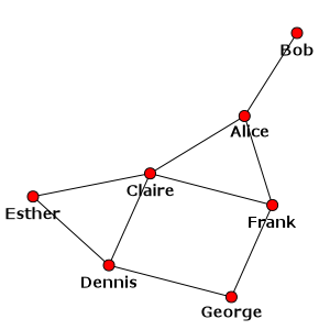
Our social network with the Kamada-Kawai layout algorithm
If you prefer to use matplotlib as a plotting engine, create an axes and use the
target argument:
>>> import matplotlib.pyplot as plt
>>> fig, ax = plt.subplots()
>>> plot(g, layout=layout, target=ax)
Hmm, this is not too pretty so far. A trivial addition would be to use the names as the
vertex labels and to color the vertices according to the gender. Vertex labels are taken
from the label attribute by default and vertex colors are determined by the
color attribute, so we can simply create these attributes and re-plot the graph:
>>> g.vs["label"] = g.vs["name"]
>>> color_dict = {"m": "blue", "f": "pink"}
>>> g.vs["color"] = [color_dict[gender] for gender in g.vs["gender"]]
>>> plot(g, layout=layout, bbox=(300, 300), margin=20)
>>> plot(g, layout=layout, bbox=(300, 300), margin=20, target=ax) # matplotlib version
Note that we are simply re-using the previous layout object here, but we also specified that we need a smaller plot (300 x 300 pixels) and a larger margin around the graph to fit the labels (20 pixels). The result is:
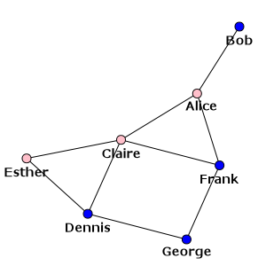
Our social network - with names as labels and genders as colors
Instead of specifying the visual properties as vertex and edge attributes, you can
also give them as keyword arguments to plot():
>>> color_dict = {"m": "blue", "f": "pink"}
>>> plot(g, layout=layout, vertex_color=[color_dict[gender] for gender in g.vs["gender"]])
This latter approach is preferred if you want to keep the properties of the visual
representation of your graph separate from the graph itself. You can simply set up
a Python dictionary containing the keyword arguments you would pass to plot()
and then use the double asterisk (**) operator to pass your specific styling
attributes to plot():
>>> visual_style = {}
>>> visual_style["vertex_size"] = 20
>>> visual_style["vertex_color"] = [color_dict[gender] for gender in g.vs["gender"]]
>>> visual_style["vertex_label"] = g.vs["name"]
>>> visual_style["edge_width"] = [1 + 2 * int(is_formal) for is_formal in g.es["is_formal"]]
>>> visual_style["layout"] = layout
>>> visual_style["bbox"] = (300, 300)
>>> visual_style["margin"] = 20
>>> plot(g, **visual_style)
The final plot shows the formal ties with thick lines while informal ones with thin lines:
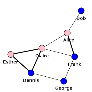
Our social network - also showing which ties are formal
To sum it all up: there are special vertex and edge properties that correspond to
the visual representation of the graph. These attributes override the default settings
of igraph (see configuring-igraph for overriding the system-wide defaults).
Furthermore, appropriate keyword arguments supplied to plot() override the
visual properties provided by the vertex and edge attributes. The following two
tables summarise the most frequently used visual attributes for vertices and edges,
respectively:
Vertex attributes controlling graph plots
Attribute name |
Keyword argument |
Purpose |
|---|---|---|
|
|
Color of the vertex |
|
|
Font family of the vertex |
|
|
Label of the vertex |
|
|
The placement of the vertex label on the circle around the vertex. This is an angle in radians, with zero belonging to the right side of the vertex. |
|
|
Color of the vertex label |
|
|
Distance of the vertex label from the vertex itself, relative to the vertex size |
|
|
Font size of the vertex label |
|
|
Drawing order of the vertices. Vertices with a smaller order parameter will be drawn first. |
|
|
Shape of the vertex. Known shapes are:
|
|
|
Size of the vertex in pixels |
Edge attributes controlling graph plots
Attribute name |
Keyword argument |
Purpose |
|---|---|---|
|
|
Color of the edge |
|
|
The curvature of the edge. Positive values
correspond to edges curved in CCW
direction, negative numbers correspond to
edges curved in clockwise (CW) direction.
Zero represents straight edges. |
|
|
Font family of the edge |
|
|
Size (length) of the arrowhead on the edge if the graph is directed, relative to 15 pixels. |
|
|
Width of the arrowhead on the edge if the graph is directed, relative to 10 pixels. |
|
|
Width of the edge in pixels |
Generic keyword arguments of plot()
These settings can be specified as keyword arguments to the plot() function
to control the overall appearance of the plot.
Keyword argument |
Purpose |
|---|---|
|
Whether to determine the curvature of the edges automatically in
graphs with multiple edges. The default is |
|
The bounding box of the plot. This must be a tuple containing the desired width and height of the plot. The default plot is 600 pixels wide and 600 pixels high. |
|
The layout to be used. It can be an instance of |
|
The top, right, bottom and left margins of the plot in pixels. This argument must be a list or tuple and its elements will be re-used if you specify a list or tuple with less than four elements. |
Specifying colors in plots
igraph understands the following color specifications wherever it expects a color (e.g., edge, vertex or label colors in the respective attributes):
- X11 color names
See the list of X11 color names in Wikipedia for the complete list. Alternatively you can see the keys of the igraph.drawing.colors.known_colors dictionary. Color names are case insensitive in igraph so “DarkBlue” can be written as “darkblue” as well.
- Color specification in CSS syntax
This is a string according to one of the following formats (where R, G and B denote the red, green and blue components, respectively):
#RRGGBB, components range from 0 to 255 in hexadecimal format. Example:"#0088ff".#RGB, components range from 0 to 15 in hexadecimal format. Example:"#08f".rgb(R, G, B), components range from 0 to 255 or from 0% to 100%. Example:"rgb(0, 127, 255)"or"rgb(0%, 50%, 100%)".
- Lists or tuples of RGB values in the range 0-1
Example:
(1.0, 0.5, 0)or[1.0, 0.5, 0].
Saving plots
igraph can be used to create publication-quality plots by asking the plot()
function to save the plot into a file instead of showing it on a screen. This can
be done simply by passing the target filename as an additional argument after the
graph itself. The preferred format is inferred from the extension. igraph can
save to anything that is supported by Cairo, including SVG, PDF and PNG files.
SVG or PDF files can then later be converted to PostScript (.ps) or Encapsulated
PostScript (.eps) format if you prefer that, while PNG files can be converted to
TIF (.tif):
>>> plot(g, "social_network.pdf", **visual_style)
igraph and the outside world
No graph module would be complete without some kind of import/export functionality
that enables the package to communicate with external programs and toolkits. igraph
is no exception: it provides functions to read the most common graph formats and
to save Graph objects into files obeying these format specifications.
The following table summarises the formats igraph can read or write:
Format |
Short name |
Reader method |
Writer method |
|---|---|---|---|
Adjacency list |
|
|
|
(a.k.a. LGL) |
|||
Adjacency matrix |
|
|
|
DIMACS |
|
|
|
DL |
|
|
not supported yet |
Edge list |
|
|
|
|
not supported yet |
|
|
GML |
|
|
|
GraphML |
|
|
|
Gzipped GraphML |
|
|
|
LEDA |
|
not supported yet |
|
Labeled edgelist |
|
|
|
(a.k.a. NCOL) |
|||
Pajek format |
|
|
|
Pickled graph |
|
|
|
As an exercise, download the graph representation of the well-known
Zachary karate club study
from this file, unzip it and try to load it into
igraph. Since it is a GraphML file, you must use the GraphML reader method from
the table above (make sure you use the appropriate path to the downloaded file):
>>> karate = Graph.Read_GraphML("zachary.graphml")
>>> summary(karate)
IGRAPH UNW- 34 78 -- Zachary's karate club network
If you want to convert the very same graph into, say, Pajek’s format, you can do it with the Pajek writer method from the table above:
>>> karate.write_pajek("zachary.net")
Note
Most of the formats have their own limitations; for instance, not all of
them can store attributes. Your best bet is probably GraphML or GML if you
want to save igraph graphs in a format that can be read from an external
package and you want to preserve numeric and string attributes. Edge list and
NCOL is also fine if you don’t have attributes (NCOL supports vertex names and
edge weights, though). If you don’t want to use your graphs outside igraph
but you want to store them for a later session, the pickled graph format
ensures that you get exactly the same graph back. The pickled graph format
uses Python’s pickle module to store and read graphs.
There are two helper methods as well: load() is a generic entry point for
reader methods which tries to infer the appropriate format from the file extension.
Graph.save() is the opposite of load(): it lets you save a graph where
the preferred format is again inferred from the extension. The format detection of
load() and Graph.save() can be overridden by the format keyword
argument which accepts the short names of the formats from the above table:
>>> karate = load("zachary.graphml")
>>> karate.save("zachary.net")
>>> karate.save("zachary.my_extension", format="gml")
Where to go next
This tutorial was only scratching the surface of what igraph can do. My long-term plans are to extend this tutorial into a proper manual-style documentation to igraph in the next chapters. In the meanwhile, check out the full API documentation which should provide information about almost every igraph class, function or method. A good starting point is the documentation of the Graph class. Should you get stuck, try asking in our Discourse group first - maybe there is someone out there who can help you out immediately.