Betweenness ¶

Betweenness¶

This example demonstrates how to visualize both vertex and edge betweenness with a custom defined color palette. We use the methods betweenness() and edge_betweenness() respectively, and demonstrate the effects on a standard Krackhardt Kite graph, as well as a Watts-Strogatz random graph.

First we import igraph and some libraries for plotting et al:

import random
import matplotlib.pyplot as plt
from matplotlib.cm import ScalarMappable
from matplotlib.colors import LinearSegmentedColormap, Normalize
import igraph as ig

Next we define a function for drawing a graph on an Matplotlib axis. We set the color and size of each vertex and edge based on the betweenness value, and also generate some color bars on the sides to see how they translate to each other. We use Matplotlib’s Normalize class to ensure that our color bar ranges are correct, as well as igraph’s rescale() to rescale the betweennesses in the interval [0, 1]:

def plot_betweenness(g, ax, cax1, cax2):
    '''Plot vertex/edge betweenness, with colorbars

    Args:
        g: the graph to plot.
        ax: the Axes for the graph
        cax1: the Axes for the vertex betweenness colorbar
        cax2: the Axes for the edge betweenness colorbar
    '''

    # Calculate vertex betweenness and scale it to be between 0.0 and 1.0
    vertex_betweenness = g.betweenness()
    edge_betweenness = g.edge_betweenness()
    scaled_vertex_betweenness = ig.rescale(vertex_betweenness, clamp=True)
    scaled_edge_betweenness = ig.rescale(edge_betweenness, clamp=True)
    print(f"vertices: {min(vertex_betweenness)} - {max(vertex_betweenness)}")
    print(f"edges: {min(edge_betweenness)} - {max(edge_betweenness)}")

    # Define mappings betweenness -> color
    cmap1 = LinearSegmentedColormap.from_list("vertex_cmap", ["pink", "indigo"])
    cmap2 = LinearSegmentedColormap.from_list("edge_cmap", ["lightblue", "midnightblue"])

    # Plot graph
    g.vs["color"] = [cmap1(betweenness) for betweenness in scaled_vertex_betweenness]
    g.vs["size"]  = ig.rescale(vertex_betweenness, (0.1, 0.5))
    g.es["color"] = [cmap2(betweenness) for betweenness in scaled_edge_betweenness]
    g.es["width"] = ig.rescale(edge_betweenness, (0.5, 1.0))
    ig.plot(
        g,
        target=ax,
        layout="fruchterman_reingold",
        vertex_frame_width=0.2,
    )

    # Color bars
    norm1 = ScalarMappable(norm=Normalize(0, max(vertex_betweenness)), cmap=cmap1)
    norm2 = ScalarMappable(norm=Normalize(0, max(edge_betweenness)), cmap=cmap2)
    plt.colorbar(norm1, cax=cax1, orientation="horizontal", label='Vertex Betweenness')
    plt.colorbar(norm2, cax=cax2, orientation="horizontal", label='Edge Betweenness')

Finally, we call our function with the two graphs:

# Generate Krackhardt Kite Graphs and Watts Strogatz graphs
random.seed(0)
g1 = ig.Graph.Famous("Krackhardt_Kite")
g2 = ig.Graph.Watts_Strogatz(dim=1, size=150, nei=2, p=0.1)

# Plot the graphs, each with two colorbars for vertex/edge betweenness
fig, axs = plt.subplots(
    3, 2,
    figsize=(7, 6),
    gridspec_kw=dict(height_ratios=(15, 1, 1)),
    )
#plt.subplots_adjust(bottom=0.3)
plot_betweenness(g1, fig, *axs[:, 0])
plot_betweenness(g2, fig, *axs[:, 1])
fig.tight_layout(h_pad=1)
plt.show()

The final output graphs are as follows:

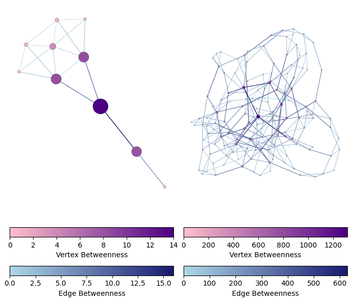
A graph visualizing the betweenness of each vertex and edge. — Vertex and edge betweenness in a Krackhardt Kite graph (left) and in a 150 node Watts-Strogatz graph (right). Edge betweenness is shown in shades of blue and vertex betweenness in shades of purple.¶

and the output for betweennesss is as follows:

vertices: 0.0 - 14.0
edges: 1.5 - 16.0
vertices: 0.0 - 1314.629277155593
edges: 1.0 - 628.2537443550603

python-igraph Manual

Betweenness ¶

Betweenness¶